Mind the Month-End

Build data pipelines that align messy inputs with planning reality

Summary

Many demand planning and S&OP teams face a familiar challenge: the data they receive does not arrive at the level of detail or cadence required for planning and decision‑making. Weekly sales data is common—especially when working with distributors, marketplaces, or external partners—yet most planning processes, dashboards, and executive reviews operate at a monthly level.

This example walks through a practical and scalable approach for bridging that gap. Using weekly sales inputs, we design a simple data pipeline that aligns weekly reporting with monthly demand planning requirements while properly handling weeks that span calendar month boundaries.

The focus is not on a specific tool or language, but on the logic and structure of the transformation: rebuilding the time dimension, explicitly defining business assumptions, and creating outputs that are reliable, auditable, and ready to support S&OP and forecasting workflows.

Weekly Sales Data

In this example, sales data is delivered weekly, with one record per week representing total sales reported on Monday. This is a common format when working with external data sources such as distributors, eCommerce platforms, or third‑party aggregators.

While this structure is perfectly reasonable for operational reporting, it presents challenges when integrating with monthly planning processes. Without additional transformation, weekly totals cannot be cleanly rolled up into months—especially when weeks cross month boundaries.

Before modeling or forecasting can begin, the data needs to be reshaped in a way that aligns with how the business reviews performance.

Step 1: Extend Weekly Sales to Daily Grain

The first step is to realign the time series to a daily structure. This does not mean estimating daily demand yet. Instead, the goal is to reconstruct the underlying calendar implied by the weekly data.

Each weekly record represents seven consecutive calendar days. By expanding the data to a daily grain, we establish a continuous time axis that allows future steps—such as allocation and aggregation—to respect month boundaries.

This step is foundational. Without restoring the daily structure, any monthly reporting built directly from weekly totals risks distortion. Importantly, no business assumptions are applied here; the sales values remain tied to their original reporting period.

daily_sales <- weekly_sales |>
  
  # Rename columns to make semantics explicit.
  # This is analogous to clarifying a source table schema in SQL.
  rename(
    week_start = Date,
    week_qty   = `Weekly Sales (Qty)`
  ) |>
  
  # Ensure week_start is treated as a proper date type.
  # Comparable to casting a VARCHAR to DATE in SQL.
  mutate(
    week_start = as.Date(week_start)
  ) |>
  
  # Expand each weekly record into the 7 calendar days it represents.
  # Conceptually similar to:
  #   - JOINing to a date dimension, or
  #   - Using GENERATE_SERIES / DATEADD logic in SQL.
  #
  # At this stage, we are only rebuilding the time axis.
  # No sales values are being redistributed yet.
  mutate(
    date = purrr::map(
      week_start,
      ~ seq(.x, .x + lubridate::days(6), by = "day")
    )
  ) |>
  tidyr::unnest(date) |>
  
  # Derive day-of-week from the calendar date,
  # then reattach the weekly quantity only to Mondays.
  #
  # This is equivalent to:
  #   CASE
  #     WHEN day_of_week = 'Monday' THEN week_qty
  #     ELSE NULL
  #   END
  #
  # Leaving non-Mondays as NULL makes the data limitation explicit.
  mutate(
    day_of_week = lubridate::wday(date, label = TRUE, abbr = FALSE),
    qty = if_else(
      day_of_week == "Monday",
      week_qty,
      NA_real_
    )
  ) |>
  
  # Select only the columns needed at the daily grain.
  # This mirrors defining a clean, consumable view in SQL.
  select(date, day_of_week, qty) |>
  
  # Order for readability and deterministic downstream behavior.
  arrange(date)

Weekly Sales Extended to Daily Grain

date	day_of_week	qty
2024-01-01	Monday	115
2024-01-02	Tuesday	NA
2024-01-03	Wednesday	NA
2024-01-04	Thursday	NA
2024-01-05	Friday	NA
2024-01-06	Saturday	NA
2024-01-07	Sunday	NA
2024-01-08	Monday	220
2024-01-09	Tuesday	NA
2024-01-10	Wednesday	NA

Step 2: Allocate Weekly Sales Across Days and Add Month Boundary

With a daily time structure in place, the next step introduces a business rule to support monthly reporting.

For this example, weekly sales are assumed to be evenly distributed across the seven days of the week. This is a simplifying assumption made to meet an immediate planning need in the absence of daily transaction data. While it may not reflect true demand patterns, it is explicit, consistent, and easy to explain to stakeholders.

Separating this allocation logic from the time expansion step is intentional. It ensures that assumptions are clearly documented and can be adjusted later—such as applying day‑of‑week weighting or replacing estimates with actual daily data when it becomes available.

At this stage, each day is also assigned to its calendar month, enabling accurate aggregation even when a single week spans multiple months.

daily_allocated_sales <- daily_sales |>
  
  # Join the weekly total back onto each daily record implicitly
  # (already present via the Monday rows in the original data).
  #
  # Apply the explicit business rule:
  # Each week’s total is divided equally across all seven days.
  mutate(
    daily_qty = if_else(
      !is.na(qty),
      qty / 7,
      NA_real_
    )
  ) |>
  
  # Propagate the allocated value to all days in the same week.
  # Conceptually similar to a window function such as:
  #   SUM(daily_qty) OVER (PARTITION BY week_start)
  group_by(lubridate::floor_date(date, "week", week_start = 1)) |>
  mutate(
    daily_qty = round(max(daily_qty, na.rm = TRUE),2)
  ) |>
  ungroup() |>
  
  # Add an explicit month boundary for downstream aggregation.
  # This mirrors deriving a month key in a date dimension table.
  mutate(
    month_beginning = lubridate::floor_date(date, "month")
  ) |> 
  select(date, day_of_week, qty, daily_qty, month_beginning)

Allocated Daily Sales

date	day_of_week	qty	daily_qty	month_beginning
2024-01-01	Monday	115	16.43	2024-01-01
2024-01-02	Tuesday	NA	16.43	2024-01-01
2024-01-03	Wednesday	NA	16.43	2024-01-01
2024-01-04	Thursday	NA	16.43	2024-01-01
2024-01-05	Friday	NA	16.43	2024-01-01
2024-01-06	Saturday	NA	16.43	2024-01-01
2024-01-07	Sunday	NA	16.43	2024-01-01
2024-01-08	Monday	220	31.43	2024-01-01
2024-01-09	Tuesday	NA	31.43	2024-01-01
2024-01-10	Wednesday	NA	31.43	2024-01-01

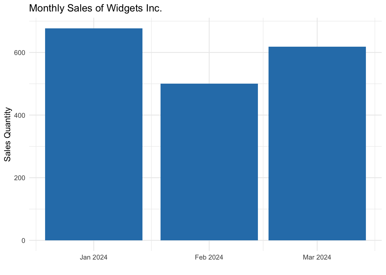
Step 3: Group Monthly and Plot

Once weekly sales have been allocated at the daily level and aligned to calendar months, monthly aggregation becomes straightforward.

This produces month‑level totals that accurately reflect demand across time, resolve cross‑month week issues, and are suitable for dashboards, reporting, forecasting models, and S&OP review materials.

The resulting visualization is not just cleaner—it is more trustworthy. Month‑over‑month comparisons now reflect actual calendar alignment rather than reporting artifacts.

monthly_sales <- daily_allocated_sales |>
  group_by(month_beginning) |>
  summarise(
    monthly_sales = sum(daily_qty),
    .groups = "drop"
  )

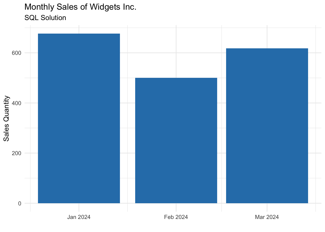
Alternate SQL Solution

While R is an excellent tool for building and validating analytical pipelines, SQL is often the most practical implementation layer for production environments. Many organizations prefer to operationalize this type of logic directly within a data warehouse, where it can be governed centrally and consumed consistently by BI tools and planning systems.

The same transformation pattern applies in SQL: reconstruct the daily time structure, apply an explicit allocation rule, and aggregate to calendar months only after alignment is complete. The result is a transparent and maintainable reporting layer that integrates cleanly into enterprise analytics stacks.

The key takeaway is that the pipeline design translates cleanly across tools. Whether implemented in R or SQL, the underlying logic remains the same.

monthly_sales_sql <- DBI::dbGetQuery(con, "
WITH expanded_days AS (
  SELECT
    ws.\"Date\" AS week_start,
    ws.\"Weekly Sales (Qty)\" AS week_qty,
    unnest(
      generate_series(
        ws.\"Date\",
        ws.\"Date\" + INTERVAL '6 days',
        INTERVAL '1 day'
      )
    )::DATE AS date
  FROM weekly_sales AS ws
),

allocated_sales AS (
  SELECT
    date,
    DATE_TRUNC('month', date)::DATE AS month_beginning,
    week_qty / 7.0 AS daily_qty
  FROM expanded_days
)

SELECT
  month_beginning,
  ROUND(SUM(daily_qty), 2) AS monthly_sales
FROM allocated_sales
GROUP BY month_beginning
ORDER BY month_beginning;
")

The result is the same as the R solution:

Conclusion

This example highlights a common but often overlooked challenge in demand planning: aligning imperfect or constrained source data with the cadence required for effective decision‑making. By rebuilding the time structure, explicitly documenting business assumptions, and separating transformation steps, the approach produces monthly sales outputs that are accurate, auditable, and ready for S&OP use.

More broadly, this illustrates how thoughtful pipeline design enables better planning outcomes even when data is limited. Rather than forcing data to fit reporting needs through shortcuts or manual adjustments, a structured transformation creates clarity and confidence for planners and leadership alike. As organizations mature their data capabilities, this same foundation can evolve—supporting more granular insights, stronger forecasts, and more resilient planning processes.